W3cubDocs
/scikit-imageskimage.restoration
Restoration algorithms, e.g., deconvolution algorithms, denoising, etc.
Create a ball kernel for restoration.rolling_ball. | |
Calibrate a denoising function and return optimal J-invariant version. | |
Cycle spinning (repeatedly apply func to shifted versions of x). | |
Denoise image using bilateral filter. | |
Apply a J-invariant version of a denoising function. | |
Perform non-local means denoising on 2D-4D grayscale or RGB images. | |
Perform total variation denoising using split-Bregman optimization. | |
Perform total variation denoising in nD. | |
Perform wavelet denoising on an image. | |
Create an ellipoid kernel for restoration.rolling_ball. | |
Robust wavelet-based estimator of the (Gaussian) noise standard deviation. | |
Inpaint masked points in image with biharmonic equations. | |
Richardson-Lucy deconvolution. | |
Estimate background intensity by rolling/translating a kernel. | |
Unsupervised Wiener-Hunt deconvolution. | |
Recover the original from a wrapped phase image. | |
Wiener-Hunt deconvolution |
-
skimage.restoration.ball_kernel(radius, ndim)[source] -
Create a ball kernel for restoration.rolling_ball.
- Parameters:
-
-
radiusint -
Radius of the ball.
-
ndimint -
Number of dimensions of the ball.
ndimshould match the dimensionality of the image the kernel will be applied to.
-
- Returns:
-
-
kernelndarray -
The kernel containing the surface intensity of the top half of the ellipsoid.
-
See also
-
skimage.restoration.calibrate_denoiser(image, denoise_function, denoise_parameters, *, stride=4, approximate_loss=True, extra_output=False)[source] -
Calibrate a denoising function and return optimal J-invariant version.
The returned function is partially evaluated with optimal parameter values set for denoising the input image.
- Parameters:
-
-
imagendarray -
Input data to be denoised (converted using
img_as_float). -
denoise_functionfunction -
Denoising function to be calibrated.
-
denoise_parametersdict of list -
Ranges of parameters for
denoise_functionto be calibrated over. -
strideint, optional -
Stride used in masking procedure that converts
denoise_functionto J-invariance. -
approximate_lossbool, optional -
Whether to approximate the self-supervised loss used to evaluate the denoiser by only computing it on one masked version of the image. If False, the runtime will be a factor of
stride**image.ndimlonger. -
extra_outputbool, optional -
If True, return parameters and losses in addition to the calibrated denoising function
-
- Returns:
-
-
best_denoise_functionfunction -
The optimal J-invariant version of
denoise_function. -
If extra_output is True, the following tuple is also returned: -
(parameters_tested, losses)tuple (list of dict, list of int) -
List of parameters tested for
denoise_function, as a dictionary of kwargs Self-supervised loss for each set of parameters inparameters_tested.
-
Notes
The calibration procedure uses a self-supervised mean-square-error loss to evaluate the performance of J-invariant versions of
denoise_function. The minimizer of the self-supervised loss is also the minimizer of the ground-truth loss (i.e., the true MSE error) [1]. The returned function can be used on the original noisy image, or other images with similar characteristics.-
Increasing the stride increases the performance of best_denoise_function -
at the expense of increasing its runtime. It has no effect on the runtime of the calibration.
References
[1]J. Batson & L. Royer. Noise2Self: Blind Denoising by Self-Supervision, International Conference on Machine Learning, p. 524-533 (2019).
Examples
>>> from skimage import color, data
>>> from skimage.restoration import denoise_tv_chambolle
>>> import numpy as np
>>> img = color.rgb2gray(data.astronaut()[:50, :50])
>>> rng = np.random.default_rng()
>>> noisy = img + 0.5 * img.std() * rng.standard_normal(img.shape)
>>> parameters = {'weight': np.arange(0.01, 0.3, 0.02)}
>>> denoising_function = calibrate_denoiser(noisy, denoise_tv_chambolle,
...                                         denoise_parameters=parameters)
>>> denoised_img = denoising_function(img)
Full tutorial on calibrating Denoisers Using J-Invariance
Full tutorial on calibrating Denoisers Using J-Invariance

-
skimage.restoration.cycle_spin(x, func, max_shifts, shift_steps=1, num_workers=None, func_kw=None, *, channel_axis=None)[source] -
Cycle spinning (repeatedly apply func to shifted versions of x).
- Parameters:
-
-
xarray-like -
Data for input to
func. -
funcfunction -
A function to apply to circularly shifted versions of
x. Should takexas its first argument. Any additional arguments can be supplied viafunc_kw. -
max_shiftsint or tuple -
If an integer, shifts in
range(0, max_shifts+1)will be used along each axis ofx. If a tuple,range(0, max_shifts[i]+1)will be along axis i. -
shift_stepsint or tuple, optional -
The step size for the shifts applied along axis, i, are::
range((0, max_shifts[i]+1, shift_steps[i])). If an integer is provided, the same step size is used for all axes. -
num_workersint or None, optional -
The number of parallel threads to use during cycle spinning. If set to
None, the full set of available cores are used. -
func_kwdict, optional -
Additional keyword arguments to supply to
func. -
channel_axisint or None, optional -
If None, the image is assumed to be a grayscale (single channel) image. Otherwise, this parameter indicates which axis of the array corresponds to channels.
Added in version 0.19:
channel_axiswas added in 0.19.
-
- Returns:
-
-
avg_ynp.ndarray -
The output of
func(x, **func_kw)averaged over all combinations of the specified axis shifts.
-
Notes
Cycle spinning was proposed as a way to approach shift-invariance via performing several circular shifts of a shift-variant transform [1].
For a n-level discrete wavelet transforms, one may wish to perform all shifts up to
max_shifts = 2**n - 1. In practice, much of the benefit can often be realized with only a small number of shifts per axis.For transforms such as the blockwise discrete cosine transform, one may wish to evaluate shifts up to the block size used by the transform.
References
[1]R.R. Coifman and D.L. Donoho. “Translation-Invariant De-Noising”. Wavelets and Statistics, Lecture Notes in Statistics, vol.103. Springer, New York, 1995, pp.125-150. DOI:10.1007/978-1-4612-2544-7_9
Examples
>>> import skimage.data
>>> from skimage import img_as_float
>>> from skimage.restoration import denoise_tv_chambolle, cycle_spin
>>> img = img_as_float(skimage.data.camera())
>>> sigma = 0.1
>>> img = img + sigma * np.random.standard_normal(img.shape)
>>> denoised = cycle_spin(img, func=denoise_tv_chambolle,
...                       max_shifts=3)

-
skimage.restoration.denoise_bilateral(image, win_size=None, sigma_color=None, sigma_spatial=1, bins=10000, mode='constant', cval=0, *, channel_axis=None)[source] -
Denoise image using bilateral filter.
- Parameters:
-
-
imagendarray, shape (M, N[, 3]) -
Input image, 2D grayscale or RGB.
-
win_sizeint -
Window size for filtering. If win_size is not specified, it is calculated as
max(5, 2 * ceil(3 * sigma_spatial) + 1). -
sigma_colorfloat -
Standard deviation for grayvalue/color distance (radiometric similarity). A larger value results in averaging of pixels with larger radiometric differences. If
None, the standard deviation ofimagewill be used. -
sigma_spatialfloat -
Standard deviation for range distance. A larger value results in averaging of pixels with larger spatial differences.
-
binsint -
Number of discrete values for Gaussian weights of color filtering. A larger value results in improved accuracy.
-
mode{‘constant’, ‘edge’, ‘symmetric’, ‘reflect’, ‘wrap’} -
How to handle values outside the image borders. See
numpy.padfor detail. -
cvalint or float -
Used in conjunction with mode ‘constant’, the value outside the image boundaries.
-
channel_axisint or None, optional -
If
None, the image is assumed to be grayscale (single-channel). Otherwise, this parameter indicates which axis of the array corresponds to channels.Added in version 0.19:
channel_axiswas added in 0.19.
-
- Returns:
-
-
denoisedndarray -
Denoised image.
-
Notes
This is an edge-preserving, denoising filter. It averages pixels based on their spatial closeness and radiometric similarity [1].
Spatial closeness is measured by the Gaussian function of the Euclidean distance between two pixels and a certain standard deviation (
sigma_spatial).Radiometric similarity is measured by the Gaussian function of the Euclidean distance between two color values and a certain standard deviation (
sigma_color).Note that, if the image is of any
intdtype,imagewill be converted using theimg_as_floatfunction and thus the standard deviation (sigma_color) will be in range[0, 1].For more information on scikit-image’s data type conversions and how images are rescaled in these conversions, see: https://scikit-image.org/docs/stable/user_guide/data_types.html.
References
[1]C. Tomasi and R. Manduchi. “Bilateral Filtering for Gray and Color Images.” IEEE International Conference on Computer Vision (1998) 839-846. DOI:10.1109/ICCV.1998.710815
Examples
>>> from skimage import data, img_as_float
>>> astro = img_as_float(data.astronaut())
>>> astro = astro[220:300, 220:320]
>>> rng = np.random.default_rng()
>>> noisy = astro + 0.6 * astro.std() * rng.random(astro.shape)
>>> noisy = np.clip(noisy, 0, 1)
>>> denoised = denoise_bilateral(noisy, sigma_color=0.05, sigma_spatial=15,
...                              channel_axis=-1)


-
skimage.restoration.denoise_invariant(image, denoise_function, *, stride=4, masks=None, denoiser_kwargs=None)[source] -
Apply a J-invariant version of a denoising function.
- Parameters:
-
-
imagendarray (M[, N[, …]][, C]) of ints, uints or floats -
Input data to be denoised.
imagecan be of any numeric type, but it is cast into a ndarray of floats (usingimg_as_float) for the computation of the denoised image. -
denoise_functionfunction -
Original denoising function.
-
strideint, optional -
Stride used in masking procedure that converts
denoise_functionto J-invariance. -
maskslist of ndarray, optional -
Set of masks to use for computing J-invariant output. If
None, a full set of masks covering the image will be used. - denoiser_kwargs:
-
Keyword arguments passed to
denoise_function.
-
- Returns:
-
-
outputndarray -
Denoised image, of same shape as
image.
-
Notes
A denoising function is J-invariant if the prediction it makes for each pixel does not depend on the value of that pixel in the original image. The prediction for each pixel may instead use all the relevant information contained in the rest of the image, which is typically quite significant. Any function can be converted into a J-invariant one using a simple masking procedure, as described in [1].
The pixel-wise error of a J-invariant denoiser is uncorrelated to the noise, so long as the noise in each pixel is independent. Consequently, the average difference between the denoised image and the oisy image, the self-supervised loss, is the same as the difference between the denoised image and the original clean image, the ground-truth loss (up to a constant).
This means that the best J-invariant denoiser for a given image can be found using the noisy data alone, by selecting the denoiser minimizing the self- supervised loss.
References
[1]J. Batson & L. Royer. Noise2Self: Blind Denoising by Self-Supervision, International Conference on Machine Learning, p. 524-533 (2019).
Examples
>>> import skimage
>>> from skimage.restoration import denoise_invariant, denoise_tv_chambolle
>>> image = skimage.util.img_as_float(skimage.data.chelsea())
>>> noisy = skimage.util.random_noise(image, var=0.2 ** 2)
>>> denoised = denoise_invariant(noisy, denoise_function=denoise_tv_chambolle)
Full tutorial on calibrating Denoisers Using J-Invariance
Full tutorial on calibrating Denoisers Using J-Invariance
-
skimage.restoration.denoise_nl_means(image, patch_size=7, patch_distance=11, h=0.1, fast_mode=True, sigma=0.0, *, preserve_range=False, channel_axis=None)[source] -
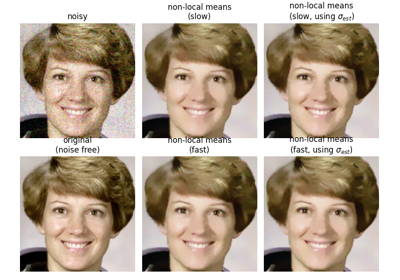
Perform non-local means denoising on 2D-4D grayscale or RGB images.
- Parameters:
-
-
image2D or 3D ndarray -
Input image to be denoised, which can be 2D or 3D, and grayscale or RGB (for 2D images only, see
channel_axisparameter). There can be any number of channels (does not strictly have to be RGB). -
patch_sizeint, optional -
Size of patches used for denoising.
-
patch_distanceint, optional -
Maximal distance in pixels where to search patches used for denoising.
-
hfloat, optional -
Cut-off distance (in gray levels). The higher h, the more permissive one is in accepting patches. A higher h results in a smoother image, at the expense of blurring features. For a Gaussian noise of standard deviation sigma, a rule of thumb is to choose the value of h to be sigma of slightly less.
-
fast_modebool, optional -
If True (default value), a fast version of the non-local means algorithm is used. If False, the original version of non-local means is used. See the Notes section for more details about the algorithms.
-
sigmafloat, optional -
The standard deviation of the (Gaussian) noise. If provided, a more robust computation of patch weights is computed that takes the expected noise variance into account (see Notes below).
-
preserve_rangebool, optional -
Whether to keep the original range of values. Otherwise, the input image is converted according to the conventions of
img_as_float. Also see https://scikit-image.org/docs/dev/user_guide/data_types.html -
channel_axisint or None, optional -
If None, the image is assumed to be a grayscale (single channel) image. Otherwise, this parameter indicates which axis of the array corresponds to channels.
Added in version 0.19:
channel_axiswas added in 0.19.
-
- Returns:
-
-
resultndarray -
Denoised image, of same shape as
image.
-
Notes
The non-local means algorithm is well suited for denoising images with specific textures. The principle of the algorithm is to average the value of a given pixel with values of other pixels in a limited neighborhood, provided that the patches centered on the other pixels are similar enough to the patch centered on the pixel of interest.
In the original version of the algorithm [1], corresponding to
fast=False, the computational complexity is:image.size * patch_size ** image.ndim * patch_distance ** image.ndim
Hence, changing the size of patches or their maximal distance has a strong effect on computing times, especially for 3-D images.
However, the default behavior corresponds to
fast_mode=True, for which another version of non-local means [2] is used, corresponding to a complexity of:image.size * patch_distance ** image.ndim
The computing time depends only weakly on the patch size, thanks to the computation of the integral of patches distances for a given shift, that reduces the number of operations [1]. Therefore, this algorithm executes faster than the classic algorithm (
fast_mode=False), at the expense of using twice as much memory. This implementation has been proven to be more efficient compared to other alternatives, see e.g. [3].Compared to the classic algorithm, all pixels of a patch contribute to the distance to another patch with the same weight, no matter their distance to the center of the patch. This coarser computation of the distance can result in a slightly poorer denoising performance. Moreover, for small images (images with a linear size that is only a few times the patch size), the classic algorithm can be faster due to boundary effects.
The image is padded using the
reflectmode ofskimage.util.padbefore denoising.If the noise standard deviation,
sigma, is provided a more robust computation of patch weights is used. Subtracting the known noise variance from the computed patch distances improves the estimates of patch similarity, giving a moderate improvement to denoising performance [4]. It was also mentioned as an option for the fast variant of the algorithm in [3].When
sigmais provided, a smallerhshould typically be used to avoid oversmoothing. The optimal value forhdepends on the image content and noise level, but a reasonable starting point ish = 0.8 * sigmawhenfast_modeisTrue, orh = 0.6 * sigmawhenfast_modeisFalse.References
[1] (1,2)A. Buades, B. Coll, & J-M. Morel. A non-local algorithm for image denoising. In CVPR 2005, Vol. 2, pp. 60-65, IEEE. DOI:10.1109/CVPR.2005.38
[2]J. Darbon, A. Cunha, T.F. Chan, S. Osher, and G.J. Jensen, Fast nonlocal filtering applied to electron cryomicroscopy, in 5th IEEE International Symposium on Biomedical Imaging: From Nano to Macro, 2008, pp. 1331-1334. DOI:10.1109/ISBI.2008.4541250
[3] (1,2)Jacques Froment. Parameter-Free Fast Pixelwise Non-Local Means Denoising. Image Processing On Line, 2014, vol. 4, pp. 300-326. DOI:10.5201/ipol.2014.120
[4]A. Buades, B. Coll, & J-M. Morel. Non-Local Means Denoising. Image Processing On Line, 2011, vol. 1, pp. 208-212. DOI:10.5201/ipol.2011.bcm_nlm
Examples
>>> a = np.zeros((40, 40))
>>> a[10:-10, 10:-10] = 1.
>>> rng = np.random.default_rng()
>>> a += 0.3 * rng.standard_normal(a.shape)
>>> denoised_a = denoise_nl_means(a, 7, 5, 0.1)
Full tutorial on calibrating Denoisers Using J-Invariance
Full tutorial on calibrating Denoisers Using J-Invariance
-
skimage.restoration.denoise_tv_bregman(image, weight=5.0, max_num_iter=100, eps=0.001, isotropic=True, *, channel_axis=None)[source] -
Perform total variation denoising using split-Bregman optimization.
Given \(f\), a noisy image (input data), total variation denoising (also known as total variation regularization) aims to find an image \(u\) with less total variation than \(f\), under the constraint that \(u\) remain similar to \(f\). This can be expressed by the Rudin–Osher–Fatemi (ROF) minimization problem:
\[\min_{u} \sum_{i=0}^{N-1} \left( \left| \nabla{u_i} \right| + \frac{\lambda}{2}(f_i - u_i)^2 \right)\]where \(\lambda\) is a positive parameter. The first term of this cost function is the total variation; the second term represents data fidelity. As \(\lambda \to 0\), the total variation term dominates, forcing the solution to have smaller total variation, at the expense of looking less like the input data.
This code is an implementation of the split Bregman algorithm of Goldstein and Osher to solve the ROF problem ([1], [2], [3]).
- Parameters:
-
-
imagendarray -
Input image to be denoised (converted using
img_as_float()). -
weightfloat, optional -
Denoising weight. It is equal to \(\frac{\lambda}{2}\). Therefore, the smaller the
weight, the more denoising (at the expense of less similarity toimage). -
epsfloat, optional -
Tolerance \(\varepsilon > 0\) for the stop criterion: The algorithm stops when \(\|u_n - u_{n-1}\|_2 < \varepsilon\).
-
max_num_iterint, optional -
Maximal number of iterations used for the optimization.
-
isotropicboolean, optional -
Switch between isotropic and anisotropic TV denoising.
-
channel_axisint or None, optional -
If
None, the image is assumed to be grayscale (single-channel). Otherwise, this parameter indicates which axis of the array corresponds to channels.Added in version 0.19:
channel_axiswas added in 0.19.
-
- Returns:
-
-
undarray -
Denoised image.
-
See also
-
denoise_tv_chambolle -
Perform total variation denoising in nD.
Notes
Ensure that
channel_axisparameter is set appropriately for color images.The principle of total variation denoising is explained in [4]. It is about minimizing the total variation of an image, which can be roughly described as the integral of the norm of the image gradient. Total variation denoising tends to produce cartoon-like images, that is, piecewise-constant images.
References
[1]Tom Goldstein and Stanley Osher, “The Split Bregman Method For L1 Regularized Problems”, https://ww3.math.ucla.edu/camreport/cam08-29.pdf
[2]Pascal Getreuer, “Rudin–Osher–Fatemi Total Variation Denoising using Split Bregman” in Image Processing On Line on 2012–05–19, https://www.ipol.im/pub/art/2012/g-tvd/article_lr.pdf
-
skimage.restoration.denoise_tv_chambolle(image, weight=0.1, eps=0.0002, max_num_iter=200, *, channel_axis=None)[source] -
Perform total variation denoising in nD.
Given \(f\), a noisy image (input data), total variation denoising (also known as total variation regularization) aims to find an image \(u\) with less total variation than \(f\), under the constraint that \(u\) remain similar to \(f\). This can be expressed by the Rudin–Osher–Fatemi (ROF) minimization problem:
\[\min_{u} \sum_{i=0}^{N-1} \left( \left| \nabla{u_i} \right| + \frac{\lambda}{2}(f_i - u_i)^2 \right)\]where \(\lambda\) is a positive parameter. The first term of this cost function is the total variation; the second term represents data fidelity. As \(\lambda \to 0\), the total variation term dominates, forcing the solution to have smaller total variation, at the expense of looking less like the input data.
This code is an implementation of the algorithm proposed by Chambolle in [1] to solve the ROF problem.
- Parameters:
-
-
imagendarray -
Input image to be denoised. If its dtype is not float, it gets converted with
img_as_float(). -
weightfloat, optional -
Denoising weight. It is equal to \(\frac{1}{\lambda}\). Therefore, the greater the
weight, the more denoising (at the expense of fidelity toimage). -
epsfloat, optional -
Tolerance \(\varepsilon > 0\) for the stop criterion (compares to absolute value of relative difference of the cost function \(E\)): The algorithm stops when \(|E_{n-1} - E_n| < \varepsilon * E_0\).
-
max_num_iterint, optional -
Maximal number of iterations used for the optimization.
-
channel_axisint or None, optional -
If
None, the image is assumed to be grayscale (single-channel). Otherwise, this parameter indicates which axis of the array corresponds to channels.Added in version 0.19:
channel_axiswas added in 0.19.
-
- Returns:
-
-
undarray -
Denoised image.
-
See also
-
denoise_tv_bregman -
Perform total variation denoising using split-Bregman optimization.
Notes
Make sure to set the
channel_axisparameter appropriately for color images.The principle of total variation denoising is explained in [2]. It is about minimizing the total variation of an image, which can be roughly described as the integral of the norm of the image gradient. Total variation denoising tends to produce cartoon-like images, that is, piecewise-constant images.
References
[1]A. Chambolle, An algorithm for total variation minimization and applications, Journal of Mathematical Imaging and Vision, Springer, 2004, 20, 89-97.
Examples
2D example on astronaut image:
>>> from skimage import color, data
>>> img = color.rgb2gray(data.astronaut())[:50, :50]
>>> rng = np.random.default_rng()
>>> img += 0.5 * img.std() * rng.standard_normal(img.shape)
>>> denoised_img = denoise_tv_chambolle(img, weight=60)
3D example on synthetic data:
>>> x, y, z = np.ogrid[0:20, 0:20, 0:20]
>>> mask = (x - 22)**2 + (y - 20)**2 + (z - 17)**2 < 8**2
>>> mask = mask.astype(float)
>>> rng = np.random.default_rng()
>>> mask += 0.2 * rng.standard_normal(mask.shape)
>>> res = denoise_tv_chambolle(mask, weight=100)
Full tutorial on calibrating Denoisers Using J-Invariance
Full tutorial on calibrating Denoisers Using J-Invariance

-
skimage.restoration.denoise_wavelet(image, sigma=None, wavelet='db1', mode='soft', wavelet_levels=None, convert2ycbcr=False, method='BayesShrink', rescale_sigma=True, *, channel_axis=None)[source] -
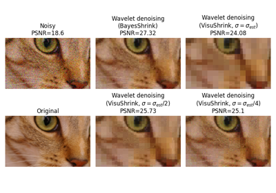
Perform wavelet denoising on an image.
- Parameters:
-
-
imagendarray (M[, N[, …P]][, C]) of ints, uints or floats -
Input data to be denoised.
imagecan be of any numeric type, but it is cast into an ndarray of floats for the computation of the denoised image. -
sigmafloat or list, optional -
The noise standard deviation used when computing the wavelet detail coefficient threshold(s). When None (default), the noise standard deviation is estimated via the method in [2].
-
waveletstring, optional -
The type of wavelet to perform and can be any of the options
pywt.wavelistoutputs. The default is'db1'. For example,waveletcan be any of{'db2', 'haar', 'sym9'}and many more. -
mode{‘soft’, ‘hard’}, optional -
An optional argument to choose the type of denoising performed. It noted that choosing soft thresholding given additive noise finds the best approximation of the original image.
-
wavelet_levelsint or None, optional -
The number of wavelet decomposition levels to use. The default is three less than the maximum number of possible decomposition levels.
-
convert2ycbcrbool, optional -
If True and channel_axis is set, do the wavelet denoising in the YCbCr colorspace instead of the RGB color space. This typically results in better performance for RGB images.
-
method{‘BayesShrink’, ‘VisuShrink’}, optional -
Thresholding method to be used. The currently supported methods are “BayesShrink” [1] and “VisuShrink” [2]. Defaults to “BayesShrink”.
-
rescale_sigmabool, optional -
If False, no rescaling of the user-provided
sigmawill be performed. The default ofTruerescales sigma appropriately if the image is rescaled internally.Added in version 0.16:
rescale_sigmawas introduced in 0.16 -
channel_axisint or None, optional -
If
None, the image is assumed to be grayscale (single-channel). Otherwise, this parameter indicates which axis of the array corresponds to channels.Added in version 0.19:
channel_axiswas added in 0.19.
-
- Returns:
-
-
outndarray -
Denoised image.
-
Notes
The wavelet domain is a sparse representation of the image, and can be thought of similarly to the frequency domain of the Fourier transform. Sparse representations have most values zero or near-zero and truly random noise is (usually) represented by many small values in the wavelet domain. Setting all values below some threshold to 0 reduces the noise in the image, but larger thresholds also decrease the detail present in the image.
If the input is 3D, this function performs wavelet denoising on each color plane separately.
Changed in version 0.16: For floating point inputs, the original input range is maintained and there is no clipping applied to the output. Other input types will be converted to a floating point value in the range [-1, 1] or [0, 1] depending on the input image range. Unless
rescale_sigma = False, any internal rescaling applied to theimagewill also be applied tosigmato maintain the same relative amplitude.Many wavelet coefficient thresholding approaches have been proposed. By default,
denoise_waveletapplies BayesShrink, which is an adaptive thresholding method that computes separate thresholds for each wavelet sub-band as described in [1].If
method == "VisuShrink", a single “universal threshold” is applied to all wavelet detail coefficients as described in [2]. This threshold is designed to remove all Gaussian noise at a givensigmawith high probability, but tends to produce images that appear overly smooth.Although any of the wavelets from
PyWaveletscan be selected, the thresholding methods assume an orthogonal wavelet transform and may not choose the threshold appropriately for biorthogonal wavelets. Orthogonal wavelets are desirable because white noise in the input remains white noise in the subbands. Biorthogonal wavelets lead to colored noise in the subbands. Additionally, the orthogonal wavelets in PyWavelets are orthonormal so that noise variance in the subbands remains identical to the noise variance of the input. Example orthogonal wavelets are the Daubechies (e.g. ‘db2’) or symmlet (e.g. ‘sym2’) families.References
[1] (1,2)Chang, S. Grace, Bin Yu, and Martin Vetterli. “Adaptive wavelet thresholding for image denoising and compression.” Image Processing, IEEE Transactions on 9.9 (2000): 1532-1546. DOI:10.1109/83.862633
[2] (1,2,3)D. L. Donoho and I. M. Johnstone. “Ideal spatial adaptation by wavelet shrinkage.” Biometrika 81.3 (1994): 425-455. DOI:10.1093/biomet/81.3.425
Examples
>>> from skimage import color, data
>>> img = img_as_float(data.astronaut())
>>> img = color.rgb2gray(img)
>>> rng = np.random.default_rng()
>>> img += 0.1 * rng.standard_normal(img.shape)
>>> img = np.clip(img, 0, 1)
>>> denoised_img = denoise_wavelet(img, sigma=0.1, rescale_sigma=True)
Full tutorial on calibrating Denoisers Using J-Invariance
Full tutorial on calibrating Denoisers Using J-Invariance
-
skimage.restoration.ellipsoid_kernel(shape, intensity)[source] -
Create an ellipoid kernel for restoration.rolling_ball.
- Parameters:
-
-
shapearray-like -
Length of the principal axis of the ellipsoid (excluding the intensity axis). The kernel needs to have the same dimensionality as the image it will be applied to.
-
intensityint -
Length of the intensity axis of the ellipsoid.
-
- Returns:
-
-
kernelndarray -
The kernel containing the surface intensity of the top half of the ellipsoid.
-
See also

Use rolling-ball algorithm for estimating background intensity
Use rolling-ball algorithm for estimating background intensity
-
skimage.restoration.estimate_sigma(image, average_sigmas=False, *, channel_axis=None)[source] -
Robust wavelet-based estimator of the (Gaussian) noise standard deviation.
- Parameters:
-
-
imagendarray -
Image for which to estimate the noise standard deviation.
-
average_sigmasbool, optional -
If true, average the channel estimates of
sigma. Otherwise return a list of sigmas corresponding to each channel. -
channel_axisint or None, optional -
If
None, the image is assumed to be grayscale (single-channel). Otherwise, this parameter indicates which axis of the array corresponds to channels.Added in version 0.19:
channel_axiswas added in 0.19.
-
- Returns:
-
-
sigmafloat or list -
Estimated noise standard deviation(s). If
multichannelis True andaverage_sigmasis False, a separate noise estimate for each channel is returned. Otherwise, the average of the individual channel estimates is returned.
-
Notes
This function assumes the noise follows a Gaussian distribution. The estimation algorithm is based on the median absolute deviation of the wavelet detail coefficients as described in section 4.2 of [1].
References
[1]D. L. Donoho and I. M. Johnstone. “Ideal spatial adaptation by wavelet shrinkage.” Biometrika 81.3 (1994): 425-455. DOI:10.1093/biomet/81.3.425
Examples
>>> import skimage.data
>>> from skimage import img_as_float
>>> img = img_as_float(skimage.data.camera())
>>> sigma = 0.1
>>> rng = np.random.default_rng()
>>> img = img + sigma * rng.standard_normal(img.shape)
>>> sigma_hat = estimate_sigma(img, channel_axis=None)
Full tutorial on calibrating Denoisers Using J-Invariance
Full tutorial on calibrating Denoisers Using J-Invariance
-
skimage.restoration.inpaint_biharmonic(image, mask, *, split_into_regions=False, channel_axis=None)[source] -
Inpaint masked points in image with biharmonic equations.
- Parameters:
-
-
image(M[, N[, …, P]][, C]) ndarray -
Input image.
-
mask(M[, N[, …, P]]) ndarray -
Array of pixels to be inpainted. Have to be the same shape as one of the ‘image’ channels. Unknown pixels have to be represented with 1, known pixels - with 0.
-
split_into_regionsboolean, optional -
If True, inpainting is performed on a region-by-region basis. This is likely to be slower, but will have reduced memory requirements.
-
channel_axisint or None, optional -
If None, the image is assumed to be a grayscale (single channel) image. Otherwise, this parameter indicates which axis of the array corresponds to channels.
Added in version 0.19:
channel_axiswas added in 0.19.
-
- Returns:
-
-
out(M[, N[, …, P]][, C]) ndarray -
Input image with masked pixels inpainted.
-
References
[1]S.B.Damelin and N.S.Hoang. “On Surface Completion and Image Inpainting by Biharmonic Functions: Numerical Aspects”, International Journal of Mathematics and Mathematical Sciences, Vol. 2018, Article ID 3950312 DOI:10.1155/2018/3950312
[2]C. K. Chui and H. N. Mhaskar, MRA Contextual-Recovery Extension of Smooth Functions on Manifolds, Appl. and Comp. Harmonic Anal., 28 (2010), 104-113, DOI:10.1016/j.acha.2009.04.004
Examples
>>> img = np.tile(np.square(np.linspace(0, 1, 5)), (5, 1))
>>> mask = np.zeros_like(img)
>>> mask[2, 2:] = 1
>>> mask[1, 3:] = 1
>>> mask[0, 4:] = 1
>>> out = inpaint_biharmonic(img, mask)


-
skimage.restoration.richardson_lucy(image, psf, num_iter=50, clip=True, filter_epsilon=None)[source] -
Richardson-Lucy deconvolution.
- Parameters:
-
-
image([P, ]M, N) ndarray -
Input degraded image (can be n-dimensional). If you keep the default
clip=Trueparameter, you may want to normalize the image so that its values fall in the [-1, 1] interval to avoid information loss. -
psfndarray -
The point spread function.
-
num_iterint, optional -
Number of iterations. This parameter plays the role of regularisation.
-
clipboolean, optional -
True by default. If true, pixel value of the result above 1 or under -1 are thresholded for skimage pipeline compatibility.
- filter_epsilon: float, optional
-
Value below which intermediate results become 0 to avoid division by small numbers.
-
- Returns:
-
-
im_deconvndarray -
The deconvolved image.
-
References
Examples
>>> from skimage import img_as_float, data, restoration
>>> camera = img_as_float(data.camera())
>>> from scipy.signal import convolve2d
>>> psf = np.ones((5, 5)) / 25
>>> camera = convolve2d(camera, psf, 'same')
>>> rng = np.random.default_rng()
>>> camera += 0.1 * camera.std() * rng.standard_normal(camera.shape)
>>> deconvolved = restoration.richardson_lucy(camera, psf, 5)

-
skimage.restoration.rolling_ball(image, *, radius=100, kernel=None, nansafe=False, num_threads=None)[source] -
Estimate background intensity by rolling/translating a kernel.
This rolling ball algorithm estimates background intensity for a ndimage in case of uneven exposure. It is a generalization of the frequently used rolling ball algorithm [1].
- Parameters:
-
-
imagendarray -
The image to be filtered.
-
radiusint, optional -
Radius of a ball-shaped kernel to be rolled/translated in the image. Used if
kernel = None. -
kernelndarray, optional -
The kernel to be rolled/translated in the image. It must have the same number of dimensions as
image. Kernel is filled with the intensity of the kernel at that position. - nansafe: bool, optional
-
If
False(default) assumes that none of the values inimagearenp.nan, and uses a faster implementation. - num_threads: int, optional
-
The maximum number of threads to use. If
Noneuse the OpenMP default value; typically equal to the maximum number of virtual cores. Note: This is an upper limit to the number of threads. The exact number is determined by the system’s OpenMP library.
-
- Returns:
-
-
backgroundndarray -
The estimated background of the image.
-
Notes
For the pixel that has its background intensity estimated (without loss of generality at
center) the rolling ball method centerskernelunder it and raises the kernel until the surface touches the image umbra at somepos=(y,x). The background intensity is then estimated using the image intensity at that position (image[pos]) plus the difference ofkernel[center] - kernel[pos].This algorithm assumes that dark pixels correspond to the background. If you have a bright background, invert the image before passing it to the function, e.g., using
utils.invert. See the gallery example for details.This algorithm is sensitive to noise (in particular salt-and-pepper noise). If this is a problem in your image, you can apply mild gaussian smoothing before passing the image to this function.
This algorithm’s complexity is polynomial in the radius, with degree equal to the image dimensionality (a 2D image is N^2, a 3D image is N^3, etc.), so it can take a long time as the radius grows beyond 30 or so ([2], [3]). It is an exact N-dimensional calculation; if all you need is an approximation, faster options to consider are top-hat filtering [4] or downscaling-then-upscaling to reduce the size of the input processed.
References
[1]Sternberg, Stanley R. “Biomedical image processing.” Computer 1 (1983): 22-34. DOI:10.1109/MC.1983.1654163
Examples
>>> import numpy as np
>>> from skimage import data
>>> from skimage.restoration import rolling_ball
>>> image = data.coins()
>>> background = rolling_ball(data.coins())
>>> filtered_image = image - background
>>> import numpy as np
>>> from skimage import data
>>> from skimage.restoration import rolling_ball, ellipsoid_kernel
>>> image = data.coins()
>>> kernel = ellipsoid_kernel((101, 101), 75)
>>> background = rolling_ball(data.coins(), kernel=kernel)
>>> filtered_image = image - background
Use rolling-ball algorithm for estimating background intensity
Use rolling-ball algorithm for estimating background intensity
-
skimage.restoration.unsupervised_wiener(image, psf, reg=None, user_params=None, is_real=True, clip=True, *, rng=None)[source] -
Unsupervised Wiener-Hunt deconvolution.
Return the deconvolution with a Wiener-Hunt approach, where the hyperparameters are automatically estimated. The algorithm is a stochastic iterative process (Gibbs sampler) described in the reference below. See also
wienerfunction.- Parameters:
-
-
image(M, N) ndarray -
The input degraded image.
-
psfndarray -
The impulse response (input image’s space) or the transfer function (Fourier space). Both are accepted. The transfer function is automatically recognized as being complex (
np.iscomplexobj(psf)). -
regndarray, optional -
The regularisation operator. The Laplacian by default. It can be an impulse response or a transfer function, as for the psf.
-
user_paramsdict, optional -
Dictionary of parameters for the Gibbs sampler. See below.
-
clipboolean, optional -
True by default. If true, pixel values of the result above 1 or under -1 are thresholded for skimage pipeline compatibility.
-
rng{numpy.random.Generator, int}, optional -
Pseudo-random number generator. By default, a PCG64 generator is used (see
numpy.random.default_rng()). Ifrngis an int, it is used to seed the generator.Added in version 0.19.
-
- Returns:
-
-
x_postmean(M, N) ndarray -
The deconvolved image (the posterior mean).
-
chainsdict -
The keys
noiseandpriorcontain the chain list of noise and prior precision respectively.
-
- Other Parameters:
-
- The keys of ``user_params`` are:
-
thresholdfloat -
The stopping criterion: the norm of the difference between to successive approximated solution (empirical mean of object samples, see Notes section). 1e-4 by default.
-
burninint -
The number of sample to ignore to start computation of the mean. 15 by default.
-
min_num_iterint -
The minimum number of iterations. 30 by default.
-
max_num_iterint -
The maximum number of iterations if
thresholdis not satisfied. 200 by default. -
callbackcallable (None by default) -
A user provided callable to which is passed, if the function exists, the current image sample for whatever purpose. The user can store the sample, or compute other moments than the mean. It has no influence on the algorithm execution and is only for inspection.
Notes
The estimated image is design as the posterior mean of a probability law (from a Bayesian analysis). The mean is defined as a sum over all the possible images weighted by their respective probability. Given the size of the problem, the exact sum is not tractable. This algorithm use of MCMC to draw image under the posterior law. The practical idea is to only draw highly probable images since they have the biggest contribution to the mean. At the opposite, the less probable images are drawn less often since their contribution is low. Finally, the empirical mean of these samples give us an estimation of the mean, and an exact computation with an infinite sample set.
References
[1]François Orieux, Jean-François Giovannelli, and Thomas Rodet, “Bayesian estimation of regularization and point spread function parameters for Wiener-Hunt deconvolution”, J. Opt. Soc. Am. A 27, 1593-1607 (2010)
https://www.osapublishing.org/josaa/abstract.cfm?URI=josaa-27-7-1593
Examples
>>> from skimage import color, data, restoration
>>> img = color.rgb2gray(data.astronaut())
>>> from scipy.signal import convolve2d
>>> psf = np.ones((5, 5)) / 25
>>> img = convolve2d(img, psf, 'same')
>>> rng = np.random.default_rng()
>>> img += 0.1 * img.std() * rng.standard_normal(img.shape)
>>> deconvolved_img = restoration.unsupervised_wiener(img, psf)

-
skimage.restoration.unwrap_phase(image, wrap_around=False, rng=None)[source] -
Recover the original from a wrapped phase image.
From an image wrapped to lie in the interval [-pi, pi), recover the original, unwrapped image.
- Parameters:
-
-
image(M[, N[, P]]) ndarray or masked array of floats -
The values should be in the range [-pi, pi). If a masked array is provided, the masked entries will not be changed, and their values will not be used to guide the unwrapping of neighboring, unmasked values. Masked 1D arrays are not allowed, and will raise a
ValueError. -
wrap_aroundbool or sequence of bool, optional -
When an element of the sequence is
True, the unwrapping process will regard the edges along the corresponding axis of the image to be connected and use this connectivity to guide the phase unwrapping process. If only a single boolean is given, it will apply to all axes. Wrap around is not supported for 1D arrays. -
rng{numpy.random.Generator, int}, optional -
Pseudo-random number generator. By default, a PCG64 generator is used (see
numpy.random.default_rng()). Ifrngis an int, it is used to seed the generator.Unwrapping relies on a random initialization. This sets the PRNG to use to achieve deterministic behavior.
-
- Returns:
-
-
image_unwrappedarray_like, double -
Unwrapped image of the same shape as the input. If the input
imagewas a masked array, the mask will be preserved.
-
- Raises:
-
- ValueError
-
If called with a masked 1D array or called with a 1D array and
wrap_around=True.
References
[1]Miguel Arevallilo Herraez, David R. Burton, Michael J. Lalor, and Munther A. Gdeisat, “Fast two-dimensional phase-unwrapping algorithm based on sorting by reliability following a noncontinuous path”, Journal Applied Optics, Vol. 41, No. 35 (2002) 7437,
[2]Abdul-Rahman, H., Gdeisat, M., Burton, D., & Lalor, M., “Fast three-dimensional phase-unwrapping algorithm based on sorting by reliability following a non-continuous path. In W. Osten, C. Gorecki, & E. L. Novak (Eds.), Optical Metrology (2005) 32–40, International Society for Optics and Photonics.
Examples
>>> c0, c1 = np.ogrid[-1:1:128j, -1:1:128j]
>>> image = 12 * np.pi * np.exp(-(c0**2 + c1**2))
>>> image_wrapped = np.angle(np.exp(1j * image))
>>> image_unwrapped = unwrap_phase(image_wrapped)
>>> np.std(image_unwrapped - image) < 1e-6   # A constant offset is normal
True

-
skimage.restoration.wiener(image, psf, balance, reg=None, is_real=True, clip=True)[source] -
Wiener-Hunt deconvolution
Return the deconvolution with a Wiener-Hunt approach (i.e. with Fourier diagonalisation).
- Parameters:
-
-
imagendarray -
Input degraded image (can be n-dimensional).
-
psfndarray -
Point Spread Function. This is assumed to be the impulse response (input image space) if the data-type is real, or the transfer function (Fourier space) if the data-type is complex. There is no constraints on the shape of the impulse response. The transfer function must be of shape
(N1, N2, ..., ND)ifis_real is True,(N1, N2, ..., ND // 2 + 1)otherwise (seenp.fft.rfftn). -
balancefloat -
The regularisation parameter value that tunes the balance between the data adequacy that improve frequency restoration and the prior adequacy that reduce frequency restoration (to avoid noise artifacts).
-
regndarray, optional -
The regularisation operator. The Laplacian by default. It can be an impulse response or a transfer function, as for the psf. Shape constraint is the same as for the
psfparameter. -
is_realboolean, optional -
True by default. Specify if
psfandregare provided with hermitian hypothesis, that is only half of the frequency plane is provided (due to the redundancy of Fourier transform of real signal). It’s apply only ifpsfand/orregare provided as transfer function. For the hermitian property seeuftmodule ornp.fft.rfftn. -
clipboolean, optional -
True by default. If True, pixel values of the result above 1 or under -1 are thresholded for skimage pipeline compatibility.
-
- Returns:
-
-
im_deconv(M, N) ndarray -
The deconvolved image.
-
Notes
This function applies the Wiener filter to a noisy and degraded image by an impulse response (or PSF). If the data model is
\[y = Hx + n\]where \(n\) is noise, \(H\) the PSF and \(x\) the unknown original image, the Wiener filter is
\[\hat x = F^\dagger \left( |\Lambda_H|^2 + \lambda |\Lambda_D|^2 \right)^{-1} \Lambda_H^\dagger F y\]where \(F\) and \(F^\dagger\) are the Fourier and inverse Fourier transforms respectively, \(\Lambda_H\) the transfer function (or the Fourier transform of the PSF, see [Hunt] below) and \(\Lambda_D\) the filter to penalize the restored image frequencies (Laplacian by default, that is penalization of high frequency). The parameter \(\lambda\) tunes the balance between the data (that tends to increase high frequency, even those coming from noise), and the regularization.
These methods are then specific to a prior model. Consequently, the application or the true image nature must correspond to the prior model. By default, the prior model (Laplacian) introduce image smoothness or pixel correlation. It can also be interpreted as high-frequency penalization to compensate the instability of the solution with respect to the data (sometimes called noise amplification or “explosive” solution).
Finally, the use of Fourier space implies a circulant property of \(H\), see [2].
References
[1]François Orieux, Jean-François Giovannelli, and Thomas Rodet, “Bayesian estimation of regularization and point spread function parameters for Wiener-Hunt deconvolution”, J. Opt. Soc. Am. A 27, 1593-1607 (2010)
https://www.osapublishing.org/josaa/abstract.cfm?URI=josaa-27-7-1593
[2]B. R. Hunt “A matrix theory proof of the discrete convolution theorem”, IEEE Trans. on Audio and Electroacoustics, vol. au-19, no. 4, pp. 285-288, dec. 1971
Examples
>>> from skimage import color, data, restoration
>>> img = color.rgb2gray(data.astronaut())
>>> from scipy.signal import convolve2d
>>> psf = np.ones((5, 5)) / 25
>>> img = convolve2d(img, psf, 'same')
>>> rng = np.random.default_rng()
>>> img += 0.1 * img.std() * rng.standard_normal(img.shape)
>>> deconvolved_img = restoration.wiener(img, psf, 0.1)
© 2019 the scikit-image team
Licensed under the BSD 3-clause License.
https://scikit-image.org/docs/0.25.x/api/skimage.restoration.html